AxeDB: Guitar Pricing Intelligence
New project for studying the used and vintage guitar markets
September 30, 2018
Baseball is an old game, and for the most part, we play it the same way today as we did several decades ago. One maneuver disrupting the old way of play in recent years in the infield shift. MLB.com defines the most common type of shift as “when three (or more, in some cases) infielders are positioned to the same side of second base (mlb.com).” Once a rare meneuver, the LA Times reported in 2015 that usage of The Shift had nearly doubled each year from 2011 to 2015 (LA Times). It seems that, in the aftermath of the early Moneyball era, where most teams have by now made significant investments in analytics, the value of strategic infield positioning has become widely appreciated.
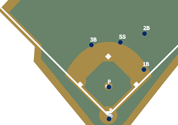 A Typical Infield Shift // mlb.com
The reasons for shifting can be many. Mike Petriello provides an excellent analysis when and why it happens in 9 things you need to know about the shift. The most obvious recipients of The Shift are lefty hitters whose spraychart shows a heavy skew toward hitting down the first baseline. It’s also clear that some teams have embraced The Shift more than others. The Astros, for example, have shifted on over 40% of plate appearances in 2018, while the Cubs barely shift at all.
The goal of this project is to see if shifts can be predicted. Predicting shifts is interesting for a few different reasons. If you’re on the defensive side and want to better know when your infield is supposed to be shifting, it may be helpful to see how likely the rest of the league would be to shift in that same situation. If you’re deciding whether to send in a pinch hitter, it will be useful to know both whether the defense is expected to shift, and how effective your batter is going to be against the maneuver. And, more generally, The Shift is just a fun maneuver that I’d like to better understand.
I will begin by collecting data from Baseball Savant, which tells us how the defense is positioned at a given point in time. From there, I’ll create features to describe game context, player identity, and player ability that will help to form predictions. Last, I’ll build five different models, ranging from simple generalized linear models to more advanced machine learning techniques, to see just how effectively The Shift can be predicted before it happens. Let’s get started.
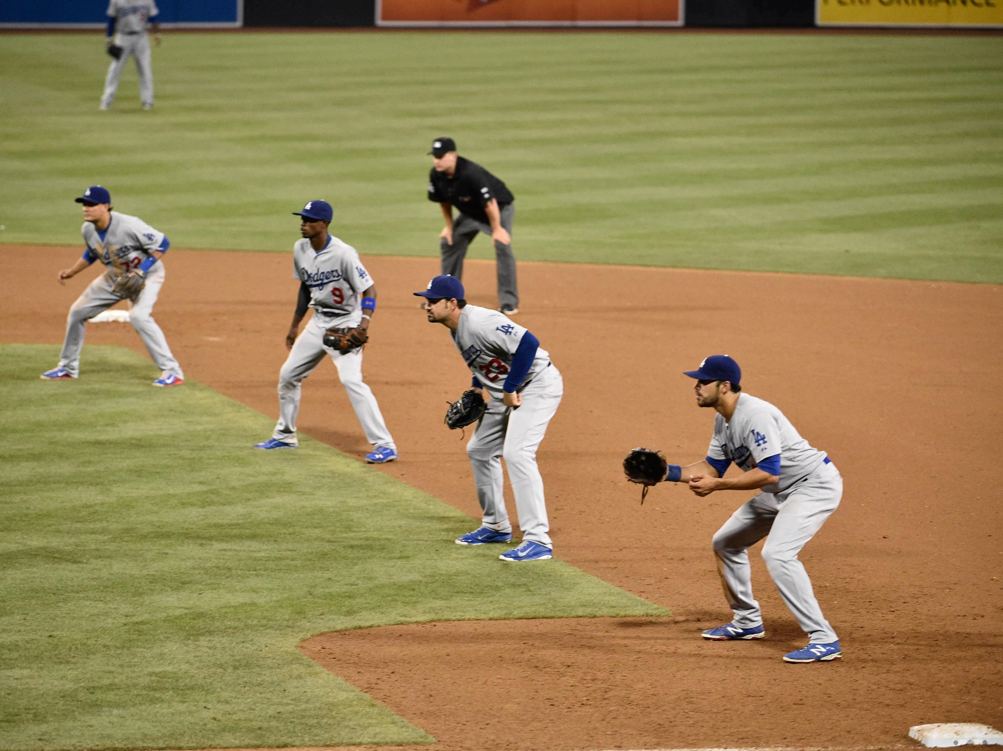 The LA Dodgers Getting Shifty // DENIS POROY / GETTY
I use pybaseball to collect statcast data. Baseball Savant has made field position classifications available since the beginning of the 2016 season, so I collect data from 2016 to present (August 2018 at the time of writing this post). Data collection is a simple one-liner.
from pybaseball import statcast
df = statcast('2016-03-25', '2018-08-17')
For a long query like this one, the scraper takes a while to complete. I recommend running this and then leaving it alone for a while. Save a copy once you have it to avoid having to re-scrape.
Now, some simple cleaning to make feature engineering and analysis possible. To start, I:
game_date into a proper datetime typegame_pk + at_bat_number)inning_topbotis_shift, defined as equaling 1 when if_fielding_alignment is equal to Infield shiftIn code, it looks like this:
# only consider regular season games
df = df.loc[df['game_type'] == 'R',]

df['game_date'] = pd.to_datetime(df['game_date'])

df['atbat_pk'] = df['game_pk'].astype(str) + df['at_bat_number'].astype(str)

# we don't have column for which team is pitching, but we know the home team pitches the top and away pitches bottom
df['team_pitching'] = np.where(df['inning_topbot']=='Top', df['home_team'], df['away_team'])
df['team_batting'] = np.where(df['inning_topbot']=='Top', df['away_team'], df['home_team'])

#is_shift == 1 if the defense was shifted at any point during the plate appearance
df['is_shift'] = np.where(df['if_fielding_alignment'] == 'Infield shift', 1, 0)
shifts = pd.DataFrame(df.groupby('atbat_pk')['is_shift'].sum()).reset_index()
shifts.loc[shifts.is_shift > 0, 'is_shift'] = 1
df = df.merge(shifts, on='atbat_pk', suffixes=('_old', ''))\

df = df[pd.notnull(df['is_shift'])]
Last, since our goal is to predict whether a shift occurred on a given plate appearance, we’ll want to reshape the data so that each record reflects a single plate appearance. Pybaseball’s statcast data comes in the lowest form of granularity offered by Baseball Savant: the individual pitch. To move the data to plate appearance-level granularity, I group by atbat_pk and select the first row of each plate appearance, which shows the game state when a player first steps up to bat. This is an oversimplification of what happens throughout the plate appearance (maybe someone stole a base, maybe there was a pitching change), but it’s a good enough representation of reality to predict how the defense would play the situation.
plate_appearances = df.sort_values(['game_date', 'at_bat_number'], ascending=True).groupby(['atbat_pk']).first().reset_index()
Taking the first row of each plate appearance isn’t enough to build useful features, of course. The pitch-level data will still be used to create features representing player ability and game context.
We’ll begin feature engineering by creating the two most obvious features that come to mind for predicting shifts: how often does the current batter get shifted against, and how often does the defensive team shift in general?
To avoid information leakage (information slipping into the model from points in time happening after the present atbat_pk), these features will be calculated using expanding means. This means that for each point in time, we’ll calculate the shift-rate from the beginning of time up until the present plate appearance, ignoring all future data that is unknown at that point in time. These features are calculated below.
# calculate an expanding mean for a given feature
def get_expanding_mean(df, featurename, base_colname):
    # arrange rows by date + PA # for each batter
    df = df.sort_values(['batter', 'game_date', 'at_bat_number'], ascending=True)
    # calculate mean-to-date at each PA's point in time
    feature_to_date = df.sort_values(['batter','game_date','at_bat_number'], ascending=True).groupby('batter')[base_colname].expanding(min_periods=1).mean()
    feature_to_date = pd.DataFrame(feature_to_date).reset_index()
    feature_to_date.columns = ['batter', 'index', featurename]
    if 'index' in df.columns:
        df = df.drop('index',1)
    # join new feature onto the original dataframe
    df = df.reset_index()
    df = pd.merge(left=df, right=feature_to_date, left_on=['batter','index'],
                                 right_on=['batter', 'index'], suffixes=['old',''])
    return df

plate_appearances = get_expanding_mean(plate_appearances, 'avg_shifted_against', 'is_shift')

# shift rate to date for each team at each point in time
plate_appearances = plate_appearances.sort_values(['team_pitching', 'game_date'], ascending=True)
shifts_to_date = plate_appearances.sort_values(['team_pitching', 'game_date'], ascending=True).groupby('team_pitching')['is_shift'].expanding(min_periods=1).mean()
shifts_to_date = pd.DataFrame(shifts_to_date).reset_index()
shifts_to_date.columns = ['team_pitching', 'index', 'def_shift_pct']
plate_appearances = plate_appearances.drop('index',1)
plate_appearances = plate_appearances.reset_index()
plate_appearances = pd.merge(left=plate_appearances, right=shifts_to_date, left_on=['team_pitching','index'], right_on=['team_pitching', 'index'], suffixes=['old',''])
Note that I created a function called get_expanding_mean in the above code chunk because later in this analysis I’ll repeat this same procedure for other features. The def_shift_pct feature requires a slightly different grouping, however, so it gets calculated without a dedicated function.
A quick check of our shift leaders looks about right. These numbers aren’t a perfect match with the ones Baseball Savant shows in its leaderboard, but my PA counts match those of Baseball Reference while Savant’s don’t. This suggests that Baseball Savant is applying some sort of filtering to its data, while my PAs are unfiltered.
| Name | Shift_Rate |
|---|---|
| chris davis | 89% |
| ryan howard | 88% |
| david ortiz | 84% |
| joey gallo | 80% |
| lucas duda | 77% |
| brandon moss | 74% |
| brian mccann | 73% |
| colby rasmus | 71% |
| adam laroche | 70% |
| mitch moreland | 69% |
Just for fun, we can also see how it broke down by season and handedness, using the raw average rather than the expanding mean.
| Name | Year | Bats | Shift_Rate |
|---|---|---|---|
| ryan howard | 2016 | L | 94% |
| chris davis | 2017 | L | 94% |
| chris davis | 2018 | L | 92% |
| chris davis | 2016 | L | 92% |
| joey gallo | 2018 | L | 89% |
| justin smoak | 2018 | L | 89% |
| colby rasmus | 2018 | L | 88% |
| mark teixeira | 2016 | L | 88% |
| carlos santana | 2018 | L | 87% |
| curtis granderson | 2018 | L | 86% |
It’s interesting to see Teixeira, a switch hitter, make an appearance now that we’re grouping by handedness. This is the first feature of many that will show that shift rate alone doesn’t tell the full story!
Applying the same procedure to teams shows who leans on this maneuver heaviest.
| Team | Shift Rate |
|---|---|
| HOU | 37% |
| TB | 34% |
| NYY | 22% |
| BAL | 22% |
| MIL | 21% |
| MIN | 18% |
| SEA | 18% |
| COL | 17% |
| CWS | 16% |
| PIT | 15% |
| SD | 14% |
| OAK | 14% |
| ARI | 14% |
| LAD | 13% |
| BOS | 13% |
| PHI | 13% |
| TOR | 11% |
| KC | 11% |
| CLE | 11% |
| DET | 11% |
| ATL | 10% |
| WSH | 10% |
| CIN | 10% |
| LAA | 9% |
| TEX | 9% |
| MIA | 8% |
| NYM | 7% |
| SF | 7% |
| STL | 5% |
| CHC | 5% |
The Astros and Rays are by far The Shift’s biggest adopters, while the Cubs, Cardinals, and a few other barely shift at all.
As we’ll see in Model #1 later in this post, these two features alone capture much of the information required in order to predict The Shift. There are, of course, reasons not to stop here and call it a day: what about batters with few historic plate appearances? These instances will surely be impacted by the instability of small sample sizes. What about switch hitters? The Teixeira example shows that shift rates lie in these cases.
In the context of shift-decisions, a batter’s identity is really a proxy for several things: his handedness, power, expected launch angle, sprint speed, and even who bats after him. If we capture some of these things directly, we may both improve our model and bring stability to its ability to predict shifts for new players.
Capturing batter and pitcher handedness is simple:
# stand (batter_bats)
plate_appearances['left_handed_batter'] = np.where(plate_appearances['stand'] == 'L', 1, 0)
# pitcher_throws
plate_appearances['pitcher_throws_left'] = np.where(plate_appearances['p_throws'] == 'L', 1, 0)
I then expand the player-profile feature set by repeating the previously-defined expanding average procedure for other variables provided by Baseball Savant: woba_value (how many points each PA contributes to wOBA), babip_value (same, but for BABIP), launch_angle, launch_speed, and hit_distance_sc. A modification of this procedure is also applied to obtain how many plate appearances we’ve seen to date for the current batter within this data, taking an expanding count instead of an expanding average.
plate_appearances = get_expanding_mean(plate_appearances, 'woba', 'woba_value')
plate_appearances = get_expanding_mean(plate_appearances, 'babip', 'babip_value')
plate_appearances = get_expanding_mean(plate_appearances, 'launch_angle', 'launch_angle')
plate_appearances = get_expanding_mean(plate_appearances, 'launch_speed', 'launch_speed')
plate_appearances = get_expanding_mean(plate_appearances, 'hit_distance_sc', 'hit_distance_sc')

# number of plate appearances observed for each player at the time of the current PA
plate_appearances = plate_appearances.sort_values(['batter', 'game_date', 'at_bat_number'], ascending=True)
pas = plate_appearances.sort_values(['batter','game_date','at_bat_number'], ascending=True).groupby('batter')['index'].expanding(min_periods=1).count()
pas = pd.DataFrame(pas).reset_index()
pas.columns = ['batter', 'index', 'pas']
plate_appearances = plate_appearances.drop('index',1)
plate_appearances = plate_appearances.reset_index()
plate_appearances = pd.merge(left=plate_appearances, right=pas, left_on=['batter','index'], right_on=['batter', 'index'], suffixes=['old',''])
Let’s check these numbers and see if they look right. First off, I’m seeing familiar faces on the wOBA leaderboard. That’s a good sign.
| Name | wOBA | PAs |
|---|---|---|
| mike trout | 0.434 | 2316 |
| aaron judge | 0.417 | 1208 |
| joey votto | 0.415 | 2561 |
| j. d. martinez | 0.413 | 2153 |
| paul goldschmidt | 0.403 | 2579 |
| bryce harper | 0.400 | 2271 |
| freddie freeman | 0.399 | 2199 |
| josh donaldson | 0.398 | 2064 |
| david ortiz | 0.397 | 1238 |
| nolan arenado | 0.395 | 2519 |
| kris bryant | 0.395 | 2366 |
Checking the leaderboard for exit velocity also looks good, showing Statcast darlings Stanton, Judge, and Ortiz all near the top during this period. These velocities are slightly lower than what we see in the MLB leaderboard, which is probably because I’m including launch angles for all plate appearance-ending events, including outs, whereas MLB is probably only including exit velocity on hits.
| Name | Exit Velocity | PAs |
|---|---|---|
| david ortiz | 92 | 1238 |
| nelson cruz | 91 | 2392 |
| pedro alvarez | 91 | 1026 |
| miguel cabrera | 90 | 1866 |
| kendrys morales | 90 | 2229 |
| giancarlo stanton | 90 | 1999 |
| aaron judge | 90 | 1208 |
| ryan zimmerman | 90 | 1636 |
| matt olson | 90 | 740 |
| josh donaldson | 90 | 2064 |
We’re off to a good start, having captured several components of the batter’s player profile, as well as measures of how often shifts occur for each batter and defense. Still missing from this data, however, is a sense of context. Shifts don’t happen in a vacuum. Priced into a shift-decision is the context of the current plate appearance (the score, men on base), and perhaps the team’s memory of how the current batter performed in previous plate appearances. If a player successfully hits out of the shift twice in a row, for example, a team may be less likely to try it a third time. This is the next category of feature I’ll create, attempting to capture the context in which a plate appearance occurs.
The first piece of context I’ll create is the base state. I’ll create four features: binary flags stating whether there’s a man on first, second, and third at the beginning of the plate appearance, and a count feature saying how many men are on base in total. Something that I haven’t tried is taking interactions of the binary flags (e.g. man on first AND second, first AND third, second AND third). I might add that in if I revisit this later.
df['man_on_first'] = np.where(df['on_1b'] > 0 , 1, 0)
df['man_on_second'] = np.where(df['on_2b'] > 0 , 1, 0)
df['man_on_third'] = np.where(df['on_3b'] > 0 , 1, 0)
df['men_on_base'] = df['man_on_first'] + df['man_on_second'] + df['man_on_third']
The result looks like this:
| on_1b | on_2b | on_3b | man_on_first | man_on_second | man_on_third | men_on_base |
|---|---|---|---|---|---|---|
| 572761 | 607231 | NaN | 1 | 1 | 0 | 2 |
| 621550 | NaN | NaN | 1 | 0 | 0 | 1 |
| 621550 | NaN | NaN | 1 | 0 | 0 | 1 |
| 621550 | NaN | NaN | 1 | 0 | 0 | 1 |
| 621550 | NaN | NaN | 1 | 0 | 0 | 1 |
Another piece of context that might matter is when the game took place. Maybe part of The Shift’s likelihood can be attributed in part to the year (teams saw it work last season, so they made it a bigger part of their strategy the following season) and the time of year (teams know less about their opponents earlier in the season, so they shift less). We already have a feature for what year it is. Let’s create one for the month as well.
df['Month'] = df['game_date'].dt.month
Next, let’s make the game’s score easier for the model to work with. We already know each team’s score, but a tree-based model needs to take two steps to make use of this, and linear model can’t gain much from it at all, because each team’s score is only interesting in the context of their opponent’s. Taking the difference between the two should help.
df['score_differential'] = df['fld_score'] - df['bat_score']
The Savant data has several categorical variables I’d like to use. To make use of these, I’ll create dummies for each one of them: for each unique value in the categorical variable, a binary feature is created as a flag for whether the variable took on that value. I’m doing this for a few features, but it will be particularly interesting for team_pitching (capturing a team’s defensive strategy) and batter (capturing the leftover features of a player’s profile that we haven’t been able to control for with the model’s other features).
The time-related features will be cast as dummies as well in case there are month- or year-specific effects that deviate from the linear relationship that a model might glean from representing these as continuous features.
Last, I’ll also create dummies from the events feature. These can’t be used directly, as they provide future-information that is not known at the beginning of the plate appearance. They can, however, be lagged and used to describe what’s happened in the batter’s most recent plate appearances, which I’ll do next.
# create dummies for pitching team, batting team, pitcher id, batter id
dummies = pd.get_dummies(plate_appearances['team_pitching']).rename(columns=lambda x: 'defense_' + str(x))
plate_appearances = pd.concat([plate_appearances, dummies], axis=1)

dummies = pd.get_dummies(plate_appearances['team_batting']).rename(columns=lambda x: 'atbat_' + str(x))
plate_appearances = pd.concat([plate_appearances, dummies], axis=1)

dummies = pd.get_dummies(plate_appearances['batter']).rename(columns=lambda x: 'batterid_' + str(x))
plate_appearances = pd.concat([plate_appearances, dummies], axis=1)

dummies = pd.get_dummies(plate_appearances['pitcher']).rename(columns=lambda x: 'pitcherid_' + str(x))
plate_appearances = pd.concat([plate_appearances, dummies], axis=1)

# bb_type dummies (to be lagged)
dummies = pd.get_dummies(plate_appearances['bb_type']).rename(columns=lambda x: 'bb_type_' + str(x))
plate_appearances = pd.concat([plate_appearances, dummies], axis=1)
plate_appearances.drop(['bb_type'], inplace=True, axis=1)

# month and year dummies
dummies = pd.get_dummies(plate_appearances['Month']).rename(columns=lambda x: 'Month_' + str(x))
plate_appearances = pd.concat([plate_appearances, dummies], axis=1)
dummies = pd.get_dummies(plate_appearances['game_year']).rename(columns=lambda x: 'Year_' + str(x))
plate_appearances = pd.concat([plate_appearances, dummies], axis=1)

# events
dummies = pd.get_dummies(plate_appearances['events']).rename(columns=lambda x: 'event_' + str(x))
plate_appearances = pd.concat([plate_appearances, dummies], axis=1)

plate_appearances.drop(['team_pitching', 'team_batting', 'home_team', 'away_team', 'inning_topbot'], inplace=True, axis=1)
Lagged variables are a way to encode information about the past. For the features we have access to during the present plate appearance (did they get on base? Did the defense shift? Was the shift successful?), we can also access them for each of the batter’s previous plate appearances. This is interesting information to send to the model, as it’s almost certainly playing through the players’ minds when someone new steps up to the plate.
The first step for creating these features is creating them at the present-time. Here’s I’ll define whether the batter got on base, whether they achieved a hit, whether the plate appearance was successful for the defensive team, and whether the plate appearance represents a shift that can be viewed as successful from the defense’s point of view. Everything else that I’ll lag already exists at present-time as a feature provided by Baseball Savant.
plate_appearances['onbase'] = plate_appearances.event_single + plate_appearances.event_single + plate_appearances.event_double + plate_appearances.event_triple

plate_appearances['hit'] = plate_appearances.event_single + plate_appearances.event_double \
                           + plate_appearances.event_triple  + plate_appearances.event_home_run

plate_appearances['successful_outcome_defense'] = plate_appearances.event_field_out + plate_appearances.event_strikeout + plate_appearances.event_grounded_into_double_play \
                        + plate_appearances.event_double_play + plate_appearances.event_fielders_choice_out + plate_appearances.event_other_out \
                        + plate_appearances.event_triple_play
plate_appearances['successful_shift'] = plate_appearances['is_shift'] * plate_appearances['successful_outcome_defense']
Missing values complicate the lagging of features, so these should be imputed before proceeding.
# simple imputations: hit location, hit_distance_sc, launch_speed, launch_angle, effective_speed,
# estimated_woba_using_speedangle, babip_value, iso_value
plate_appearances.loc[pd.isna(plate_appearances.hit_location), 'hit_location'] = 0
plate_appearances.loc[pd.isna(plate_appearances.hit_distance_sc), 'hit_distance_sc'] = 0
plate_appearances.loc[pd.isna(plate_appearances.launch_speed), 'launch_speed'] = 0
plate_appearances.loc[pd.isna(plate_appearances.launch_angle), 'launch_angle'] = 0
plate_appearances.loc[pd.isna(plate_appearances.effective_speed), 'effective_speed'] = 0
plate_appearances.loc[pd.isna(plate_appearances.estimated_woba_using_speedangle), 'estimated_woba_using_speedangle'] = 0
plate_appearances.loc[pd.isna(plate_appearances.babip_value), 'babip_value'] = 0
plate_appearances.loc[pd.isna(plate_appearances.iso_value), 'iso_value'] = 0
plate_appearances.loc[pd.isna(plate_appearances.woba_denom), 'woba_denom'] = 1
plate_appearances.loc[pd.isna(plate_appearances.launch_speed_angle), 'launch_speed_angle'] = 0
Now for the fun part. First sort everything chronologically for each batter. Define which columns should be lagged, and how many plate appearances into the past we should look. Then, for each lagged feature, and for each number of PAs into the past t that should be captured, group by the batter’s id and shift the column up t positions.
# finally: lag things for a fuller sense of context
plate_appearances = plate_appearances.sort_values(['batter', 'game_date', 'at_bat_number'], ascending=True)
cols_to_lag = ['is_shift', 'onbase', 'hit', 'successful_outcome_defense', 'successful_shift',
              'woba_value', 'launch_speed', 'launch_angle', 'hit_distance_sc', 'bb_type_popup', 'bb_type_line_drive',
               'bb_type_ground_ball', 'bb_type_fly_ball']

# how many PAs back to we want to consider?
lag_time = 5
for col in cols_to_lag:
    for time in range(lag_time):
        feature_name = col + '_lag' + '_{}'.format(time+1)
        plate_appearances[feature_name] = plate_appearances.groupby('batter')[col].shift(time+1)
Since this shifts the column t positions forward in time, the first t rows for each player will be missing the lagged value. For every other point in time, however, we will now know what happened up to t plate appearances ago.
There are two things to consider when picking how many plate appearances into the past we should look. The first is that each additional point in time we choose for this window will provide some extra information, but that the amount of information we gain will decrease as the size of this window increases.
Big-I “information” in this case can be described as the extent to which the added feature surprises us. Knowing nothing about past plate appearances, adding one point of past information tells us something we didn’t know before. Knowing whether the defense shifted at t-1 tells us a lot about whether they’ll shift the next time, greatly improving our prediction at time t. Compared to what we knew without it, point t-1 surprised us. Extending this one point in time further into the past, point t-2 tells us something new, but it’s not quite as surprising, as t-1 already captures a lot of what t-2 is telling us on average. Pair these diminishing returns with the feature bloat that they bring, and it’s probably not worth lagging more than a few points in time into the past.
The second thing to consider is that the more you lag, the more missing values your data will have. I chose to lag 5 points into the past, so my lagged features will be missing values for each batter’s first 5 plate appearances. This means I’ll have to throw out each player’s first five plate appearances in order to feed this data to a model. This doesn’t feel like much of a sacrifice at t=5, but it’s another reason to avoid lagging too far into the past.
Here’s an example of what this looks like for the is_shift lags for Mitch Moreland’s first 8 plate appearances. Note that NaNs in rows 1 - 5, and how a shift stays represented in the data for five plate appearances by moving through the lagged features as time progresses.
| PA Number | is_shift | is_shift_lag_1 | is_shift_lag_2 | is_shift_lag_3 | is_shift_lag_4 | is_shift_lag_5 |
|---|---|---|---|---|---|---|
| 1 | 1 | NaN | NaN | NaN | NaN | NaN |
| 2 | 1 | 1 | NaN | NaN | NaN | NaN |
| 3 | 0 | 1 | 1 | NaN | NaN | NaN |
| 4 | 0 | 0 | 1 | 1 | NaN | NaN |
| 5 | 1 | 0 | 0 | 1 | 1 | NaN |
| 6 | 1 | 1 | 0 | 0 | 1 | 1 |
| 7 | 1 | 1 | 1 | 0 | 0 | 1 |
| 8 | 0 | 1 | 1 | 1 | 0 | 0 |
I chose t=5 somewhat arbitrarily. It seemed like enough to capture most of what will be in a player’s recent memory without exploding the model’s feature space to the point of complicating the training process. There’s room for experimentation here, though, which I’d encourage for anyone planning on using a model like this in a serious way.
That was a marathon, but we now have an interesting and expansive set of features to build models on, covering player profile, ability, and context. Let’s predict some shifts.
My general modeling approach is to use k-fold cross validation for a few different models. For this reason, a fair model evaluation will necessitate a training set (which will be broken into folds for multiple train/test splits) and a holdout set, which will only be accessed once a final and “best” model is selected, for a blind evaluation of its performance.
Given the 655,847 plate appearances in this data, a 3-fold cross validation will entail 349,784 training and 174,893 test samples for each of its three train/test splits, with 131,170 samples remaining in the 20% holdout set to assess model performance.
This is set up as follows:
train_percent = .8
train_samples = int(plate_appearances.shape[0] * train_percent)
holdout_samples = int(plate_appearances.shape[0] * (1 - train_percent))

y = plate_appearances['is_shift']
X = plate_appearances.drop(['is_shift', 'batter', 'pitcher'], 1)

X_train = X[:train_samples]
X_holdout = X[train_samples:]
y_train = y[:train_samples]
y_holdout = y[train_samples:]
For the sake of my own sanity, I’m going to sacrifice some of my models’ accuracy in the name of cutting down their training time by doing some preliminary feature selection. This isn’t the only way to do this, but my method of choice is to train a random forest and use Scikit-Learn’s built in gini importances in order to rank features by their importance to the model. Everything with an importance above a cutoff value will remain in the model, while the other features will be thrown out.
#train a random forest
n_estimator = 100
rf = RandomForestClassifier(max_depth=3, n_estimators=n_estimator, n_jobs=3, verbose=2)
rf.fit(X_train, y_train)

# use random forest's feature importances to select only important features
sfm = SelectFromModel(rf, prefit=True, threshold=0.0001)

# prune unimportant features from train and holdout dataframes
feature_idx = sfm.get_support()
feature_names = X_train.columns[feature_idx]
X_train = pd.DataFrame(sfm.transform(X_train))
X_holdout = pd.DataFrame(sfm.transform(X_holdout))
X_train.columns = feature_names
X_holdout.columns = feature_names
As is common in high dimensional data, these data had several sparsely-populated features that contained very little information about shift decisions. Chief among these low-information features were the pitcher and batter dummies, which populated the majority of the feature space. After dropping low-importance features, only a few of these player ID variables remained.
For an idea about which features the final Random Forest model used in this project found most important, the ranked Gini importances of its top features are shown here:
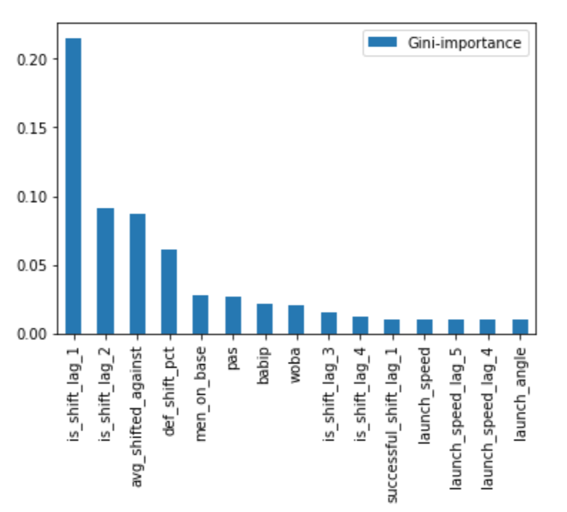 Ranked Feature Importances from Random Forest Model
This shows that most of the information is captured by whether the defense shifted in recent plate appearances, as the three most important features are the two most recent shift-lags and the batter’s historic shifted-against rate. After that, there’s a noticeable dropoff between the shift-related features and those describing game state, player ability, and the more-distant past.
Trimming low-importance features takes us from 2,781 to 109 features, and reduces the training time of a 60-model XGBoost parameter search from 4 hours down to just 29 minutes. The cost of this is essentially nonexistent. In a first-pass at modeling this, the 2,700-feature XGBoost model obtained an AUC score of 0.911 and the 100-feature model scored 0.910. That’s a tradeoff I will happily take.
A model is only interesting in the context of what it’s competing against. A good baseline to start with is the worst model imaginable, taking zero covariates into consideration. The no-model model simply guesses the majority class 100% of the time. In this case, the classes are imbalanced, so even no-model scores well on accuracy. Here y_train.mean() shows that 14% of plate appearances contain The Shift, so a model that only guesses no shift (y = 0) will be correct 86% of the time. Any lift in accuracy above this point will be learned from data.
A reasonable next step from this is a simple model using the bare-minimum set of features needed to understand The Shift. In this case, the model is logistic regression, and the only features are:
These two features collectively capture a lot of information, giving an understanding of what we know about The Shift without any machine learning or clever feature engineering.
A few lines get us this improved logistic baseline:
lr = LogisticRegression(n_jobs=3)
lr.fit(X_train[['avg_shifted_against', 'def_shift_pct']], y_train)

y_pred_lr = lr.predict_proba(X_test[['avg_shifted_against', 'def_shift_pct']])[:, 1]
fpr_lr, tpr_lr, _ = roc_curve(y_test, y_pred_lr)
So: knowing only how often a batter is shifted against and how often the defense shifts in general, how well can we predict The Shift?
It turns out, the answer is “pretty well.”
This model achieves 88.6% out of sample accuracy and an AUC score of 0.887. The accuracy is slightly better than that of the no-model model, and the high AUC score shows that the model has learned a decent amount.
Given that we have 88.6% accuracy and 0.887 AUC knowing only these two things, we can tell that a large amount of the mental calculus going into a shift-decision can be summarized by the batter’s identity and the defense’s overarching philosophy toward this maneuver.
With two baselines established, the next step in the ladder of modeling complexity is a logistic model with two improvements from the previous:
LogisticRegressionCV to shrink the model’s weights toward zero, optimizing the shrinkage parameter to maximize accuracy on unseen datalr2 = LogisticRegressionCV(n_jobs=3)
lr2.fit(X_train, y_train)
y_pred_lr2 = lr2.predict_proba(X_test)[:, 1]
fpr_lr2, tpr_lr2, _ = roc_curve(y_test, y_pred_lr2)
This model performs much better than the simple logit, with an accuracy of 92.2% and an AUC score of 0.940. This is a big leap in performance, considering how close the previous model had already come to perfect accuracy and AUC. This comes at the cost of training time, which is increased due to the larger feature space and tuning of the regularization parameter over three folds.
Next I’ll cross an arbitrary boundary between what one might call purely statistical modeling and Machine Learning with something tree-based. I opt to use a random forest classifier here because it’s a good baseline for how far machine learning will take you in a modeling task. It’s hard to overfit, relatively quick to train, and typically serves as a good hint for whether it’s worth going all-in on a more powerful nonparametric modeling approach such as gradient boosting or a neural network.
Since this and the following model are slower to train and have more tunable parameters than the previously-used linear models, I’ll first build a timer function and a modeling function so I can be consistent with how the best versions of these models are selected.
I’ll use randomized parameter search to find an optimal set of hyperparameters. This has been shown to produce superior results to grid search in less time for two reasons: it doesn’t need to run an exhaustive search to explore the parameter space, and it can explore the space more completely by sampling parameter values from distributions, rather than a grid search’s approach of sampling only from user-specified lists of values. In my implementation, I’ll accept a draws parameter, for how many draws from the sample distributions should be tested while exploring the feature space, and a folds parameter, for how many folds we’d like to cross validate over.
def timer(start_time=None):
    if not start_time:
        start_time = datetime.now()
        return start_time
    elif start_time:
        thour, temp_sec = divmod((datetime.now() - start_time).total_seconds(), 3600)
        tmin, tsec = divmod(temp_sec, 60)
        print('\n Time taken: %i hours %i minutes and %s seconds.' % (thour, tmin, round(tsec, 2)))
    return None

def model_param_search(model, param_dict, fit_dict=None, folds=3, draws=20):
    skf = StratifiedKFold(n_splits=folds, shuffle = True, random_state = 1001)
    random_search_model = RandomizedSearchCV(model, param_distributions=param_dict,
                                   fit_params=fit_dict, n_iter=draws,
                                   scoring='roc_auc', n_jobs=1, cv=skf.split(X_train,y_train), verbose=10,
                                   random_state=1001)
    start_time = timer(None)
    random_search_model.fit(X_train, y_train)
    timer(start_time)
    print('\n All results:')
    print(random_search_model.cv_results_)
    print('\n Best estimator:')
    print(random_search_model.best_estimator_)
    print('\n Best hyperparameters:')
    print(random_search_model.best_params_)
    return random_search_model
Applying this to the random forest model, I’ll draw from a uniform distribution to tune the number of trees used in the forest, simultaneously toggling the number of features considered in each tree, the criterion used for assessing the quality of decision-splits, and a flag for whether to use down-sampling to overcome the training data’s imbalanced classes caused the The Shift’s rarity.
rf_params = {
    'n_estimators': st.randint(4,200),
    'max_features': ['sqrt', .5,  1],
    'criterion': ['entropy', 'gini'],
    'class_weight': ['balanced', None]
}

random_search_rf = model_param_search(model=RandomForestClassifier(verbose=0, n_jobs=4), param_dict=rf_params, draws=10)
In the interest of time, I sample only ten times from this search space while training over three folds, equaling 30 models trained in total. Given access to better hardware, I’d feel more comfortable with the final model having doubled this number, but alas, my 12” macbook wasn’t having it.
This ended up taking just over three hours to complete, with the following as its most successful set of parameters:
{
	'class_weight': None,
	'criterion': 'entropy',
	'max_features': 0.5,
	'n_estimators': 184
}
The result was a model with 92.9% accuracy and 0.957 AUC score. This marks an improvement from the logistic score, but not as big a jump as we’d achieved by introducing contextual features in the previous step.
The last solo-model I’ll train is a gradient boosting machine using XGBoost. This is a step up from the Random Forest in complexity, and usually a good choice for a final, best model in a project like this, evidenced by its almost unmatched success in Kaggle competitions. The obvious benefit of gradient boosting is that it’s usually able to produce superior results to other tree-based methods by placing increased weights on the samples it has the most trouble classifying (general info here), but it comes at the cost of having more hyperparameters to tune and a greater propensity to overfit. In my experience it’s generally 2x the work for a 1 - 5% performance boost over a random forest. In this case, my goal is accuracy, so I’ll take it.
My approach to training this model is similar to the previous: I conduct a randomized parameter search, this time taking 20 draws from a set of parameter distributions and cross validating over three folds, making for 60 models in total.
The hyperparameters I tune are:
# using proper random search setup instead of a set list of available options
xgb_params = {
    'min_child_weight': st.randint(1,10),
    'gamma': [0], #st.uniform(0, 5),
    'subsample': st.uniform(0.5, 0.5),
    'colsample_bytree': st.uniform(0.4, 0.6),
    'max_depth': st.randint(2, 10),
    'learning_rate': st.uniform(0.02, 0.2),
    'reg_lambda': [1, 10, 100],
    'n_estimators': st.randint(10, 1000)
}
min_child_weight controls complexity by requiring a minimum weight in order to make a new split in a tree. gamma and reg_lambda perform similar functions, where reg_lambda is an L2 regularizer on the model’s weights and gamma is the minimum loss reduction needed to add a new split to a tree. subsample is the percentage of rows that a tree is allowed to see, and colsample_bytree does the same thing, but for features rather than records. Last, max_depth defines the depth of each tree, n_estimators defines the number of trees to be built, and learning_rate sets the pace at which the model is allowed to update its weights at each step during gradient descent.
To manage overfitting, I also pass a dictionary of model-fitting parameters to define an early stopping rule. This just means that, for each model, I will halt training and select the best version of the model so far if the test loss doesn’t improve for ten consecutive iterations. Assuming the out of sample loss score follows a convex pattern, this means we can find the best model without overfitting.
# create a separate holdout set for XGB early stopping
train_percent = .9
train_samples_xgb = int(X_train.shape[0] * train_percent)
test_samples_xgb = int(X_train.shape[0] * (1 - train_percent))

X_train_xgb = X_train[:train_samples_xgb]
X_test_xgb = X_train[train_samples_xgb:]
y_train_xgb = y_train[:train_samples_xgb]
y_test_xgb = y_train[train_samples_xgb:]

xgb_fit = {
    'eval_set': [(X_test_xgb, y_test_xgb)],
    'eval_metric': 'auc',
    'early_stopping_rounds': 10
}

xgb = XGBClassifier(objective='binary:logistic',
                    silent=False, nthread=3)

random_search_xgb = model_param_search(model=xgb, param_dict=xgb_params, fit_dict = xgb_fit)
One additional step I take in the above code chunk is that I create a new, additional holdout set to use for this model’s training. I’m doing this because XGBoost’s early stopping method doesn’t work well within sklearn’s randomized parameter search module. While an sklearn model will use each cross validation iteration’s holdout fold for parameter tuning using RandomizedSearchCV, XGBoost requires a static evaluation set to be passed to its eval_set parameter. It would be cheating to pass the holdout set used for final model evaluation into this parameter, so I create an intermediate holdout set out of our training set to give the model something to evaluate against for parameter tuning.
A better approach would be to define the model’s cross validation and parameter search manually in this case, passing each iteration’s holdout fold as the eval set during cross validation. This would have the benefit of letting the model see 100%, rather than 90%, of the training data, and also of using all of the training data for evaluation rather than just our new and static 10% holdout set. Given more time or a more serious use case for the model, I’d recommend going this route.
Training 60 models isn’t quick, so I recommend setting this up and forgetting it for a while. About 3 hours later, the best-performing hyperparameters were:
{
	'colsample_bytree': 0.8760738910546659,
	'gamma': 0,
	'learning_rate': 0.21627727424943,
	'max_depth': 8,
	'min_child_weight': 7,
	'n_estimators': 408,
	'reg_lambda': 10,
	'subsample': 0.8750373222444883
}
None of these values are at the extreme ends of the distributions defined for the parameter search, so I feel safe in saying that the feature space has been explored adequately.
The resulting model has 93.2% accuracy and 0.957 AUC score. As expected, this is better than the random forest, but not by a lot.
The last model is a simple ensemble of the three best models. The intuition behind this is that each model has learned something from the data, and that one model’s deficiencies may be corrected by the strengths of the others. Regression toward the mean is your friend when all models involved are good models.
In this case, there’s the additional benefit that we have three very-different models: a generalized linear model, a random forest, and a gradient boosting machine. The benefits of ensembling are greatest when the models aren’t highly correlated.
I’ll weight the models in order of performance, giving more attention to the XGBoost model and less to the logistic model.
# an ensemble of the three best models
y_pred_ensemble = (3*y_pred_xgb + 2*y_pred_rf + y_pred_lr2) / 6
fpr_ens, tpr_ens, _ = roc_curve(y_holdout, y_pred_ensemble)
Another approach I tried unsuccessfully was model stacking. In this approach I took the outputs of these same three models and fed them to a logistic regression model. To my surprise, this model-of-models approach didn’t perform any better than this simpler ensembling method, so I’m not going to give its results any further attention here.
Because The Shift is relatively uncommon, I lean on AUC score as my metric of choice. Accuracy is more interpretable as a metric, so I will report on that too, but AUC is the most fair way to compare these models against one another.
| Model | AUC | Accuracy |
|---|---|---|
| Logistic Without Context | 0.887 | 88.6% |
| Logistic With Context | 0.940 | 92.2% |
| Random Forest | 0.957 | 92.9% |
| XGBoost | 0.957 | 93.2% |
| Average of Models | 0.959 | 93.2% |
| Stacked Models | 0.955 | 92.8% |
My first thought when seeing this is that it’s a good reminder that most of your gains in any modeling task come from feature engineering. Using hand-crafted features improves the logistic AUC from 0.88 to 0.94, and gives it nearly four percentage points of increased accuracy. That’s a huge gain in a problem where only 14% of observations come from the minority class that we’re trying to predict. Moving from the logistic model to more complicated models, however, shows smaller gains. The features got us most of the way there, and machine learning provided the incremental “last mile” gains needed to move from a decent model to an optimal one.
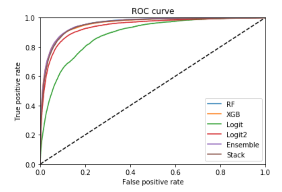 AUC Scores for All Models
The different models’ ROC curves show this visually. There’s a huge gain in going from just the two main variables to including all of our hand-crafted features. After that, there are some gains to show for using more advanced modeling techniques, but the gains are comparatively small.
The best model here is the average of the three best standalone models, which provides an AUC score of almost 0.96 and an accuracy above 93%. Those are both really good scores, indicating that these models have learned a lot from the underlying data.
One thing I noticed that can make the modeling experience much better in this case is to come up with a criterion for dropping features that don’t provide much information to the model. An approach I found success with was to use sklearn’s SelectFromModel function in conjunction with RandomForestClassifier’s built-in gini importance scores. Another approach that may have worked here would have been to sue an L1-penalized logistic regression model, optimize the shrinkage parameter, and thrown out the features whose weights had shrunk to zero.
Something that isn’t in this model, which I wish I’d used, was each team’s record at the time of each game. I suspect that strategic positioning happens less when the playoffs are out of reach. This could be captured by using win-percentage and games-left-in-season as features in the model, and I suspect this would provide some lift in the final results.
Another thing I wish I’d been able to capture in this model is a player’s sprint speed. I don’t believe this is present in the data that I was working with, but I would guess that this plays at least a minor role when a team decides whether to shift.
One last idea this leaves untested is whether I didn’t go far enough in exploring the idea of modeling this as a sequence learning problem. Providing lagged features clearly gives considerable lift over only using static features. What would happen if we represented players’ atbat histories as sequences and trained an LSTM on the relationship between these histories and their corresponding defensive positioning? The data are reasonably large, so it’s not completely crazy to think that this approach would work.
All in all, I’m pretty happy with how this turned out. Taking player profile, ability, and game context into account, these models show that we can predict The Shift with over 93% accuracy, with a near-perfect AUC score of 0.959. A perfect model is probably impossible here, but I’d like to think up a few new features that can help to fix these final 7% of missed predictions. If I come up with anything interesting, I’ll be updating this post.
New project for studying the used and vintage guitar markets
This post explores four algorithms for solving the multi-armed bandit problem (Epsilon Greedy, EXP3, Bayesian UCB, and UCB1), with implementations in Python ...
Multi-armed bandit algorithms are seeing renewed excitement, but evaluating their performance using a historic dataset is challenging. Here’s how I go about ...
An analysis of auction dynamics in client-side header bidding
Using machine learning to predict strategic infield positioning using statcast data and contextual feature engineering.
A quick tutorial on fetching MLB win-loss data with pybaseball and cleaning and visuzlizing it with the tidyverse (dplyr and ggplot).
Tanking becomes a hot topic each season once it becomes apparent which of the NBA’s worst teams will be missing the playoffs. In this post I address the valu...
I’ve been borderline obsessed with the eephus pitch for some time now. Every time I see a player pull this pitch out of their arsenal I become equal parts ex...
For the past three months I have had the exciting opportunity to intern as a data scientist at Major League Baseball Advanced Media, the technology arm of ML...
Throughout my baseball-facing work at MLB Advanced Media, I came to realize that there was no reliable Python tool available for sabermetric research and adv...
A collection of some of my favorite books. Business, popular economics, stats and machine learning, and some literature.
Each cup of coffee I have consumed in the past 5 months has been logged on a spreadsheet. Here’s what I’ve learned by data sciencing my coffee consumption.
Literature is a tricky area for data science. Think of your five favorite books. What do they have in common? Some may share an author or genre, but besides ...
Probabilistic modeling on NFL field goal data. Applying logistic regression, random forests, and neural networks in R to measure contributing factors of fiel...