Offline Evaluation of Multi-Armed Bandit Algorithms in Python using Replay

January 20, 2020

Multi-armed bandit algorithms are seeing renewed excitement in research and industry. Part of this is likely because they address some of the major problems internet companies face today: a need to explore a constantly changing landscape of (news articles, videos, ads, insert whatever your company does here) while avoiding wasting too much time showing low-quality content to users. Part of this is also may be related to advancements in a class of personalizable bandit algorithms, contextual bandits, which pair nicely with recent advances in reinforcement learning.

In either case, bandit algorithms are notoriously hard to work with using real-world datasets. Being online learning algorithms, there’s some nuance to evaluating and tuning them offline without exposing an untested algorithm to real users in a live production setting. It’s important to be able to evaluate these algorithms offline, however, for at least two reasons. First, not everybody has access to a production environment with the scale required to experiment with an online learning algorithm. And second, even those who do have a popular product at their disposal should probably be a little more careful with it than blindly throwing algorithms into production and hoping they’re successful.

Whether you’re a hobbyist wanting to experiment with bandits in your free time or someone at a big company who wants to optimize an algorithm before exposing it to users, you’re going to need to evaluate your model offline. This post discusses some methods I’ve found useful in doing this.

Creating a Dataset

For this post I’m using the Movielens 25m dataset. This dataset includes roughly 25m movie ratings for 27,000 movies provided by 138,000 users of the University of Minnesota’s Movielens service.

To cast this dataset as a bandit problem, we’ll pretend that a user rated every movie that they saw, ignoring any sort of non-rating bias that may exist. Since bandit algorithms have a time component to them (they can only see data from the past, which is constantly updated as the model learns), I shuffle the data and create a pseudo-timestamp value (which is really just a row number, but this is enough for a simulated bandit environment). To further simplify the problem, I redefine the problem from being a 0-5 star rating problem to a binary problem of modeling whether or not a user “liked” a movie. I define a rating of 4.5 stars or more as a “liked” movie, and anything else as a movie the user didn’t like. To further aid learning, I discard movies from the dataset with less than 1,500 ratings. Too few ratings to a movie can cause the model to get stuck in offline evaluation, for reasons that will make more sense soon.

The end result is a dataset of roughly 6.5 million binary like/no-like movie ratings of the form:

\([timestamp, userId, movieId, liked]\).

I do this by constructing the following get_ratings_25m function, which creates the dataset and turns it into a viable bandit problem.

def read_movielens_25m():
    ratings = pd.read_csv('ratings.csv', engine='python')
    movies = pd.read_csv('movies.csv', engine='python')
    links = pd.read_csv('links.csv', engine='python')
    movies = movies.join(movies.genres.str.get_dummies().astype(bool))
    movies.drop('genres', inplace=True, axis=1)
    df = ratings.join(movies, on='movieId', how='left', rsuffix='_movie')
    return df

def preprocess_movielens_25m(df, min_number_of_reviews=20000):
    # remove ratings of movies with < N ratings. too few ratings will cause the recsys to get stuck in offline evaluation
    movies_to_keep = pd.DataFrame(df.movieId.value_counts())\
        .loc[pd.DataFrame(df.movieId.value_counts())['movieId']>=min_number_of_reviews].index
    df = df.loc[df['movieId'].isin(movies_to_keep)]
    # shuffle rows to debias order of user ids
    df = df.sample(frac=1)
    # create a 't' column to represent time steps for the bandit to simulate a live learning scenario
    df['t'] = np.arange(len(df))
    df.index = df['t']
    # rating >= 4.5 stars is a 'like', < 4 stars is a 'dislike'
    df['liked'] = df['rating'].apply(lambda x: 1 if x >= 4.5 else 0)
    return df

def get_ratings_25m(min_number_of_reviews=20000):
    df = read_movielens_25m()
    df = preprocess_movielens_25m(df, min_number_of_reviews=20000)
    return df

Setting Up a Simulation Environment

Now that we have a dataset, we need to construct a simulation environment to use for training the bandit. A traditional ML model is trained by building a representative training and test set, where you train and tune a model on the training set and evaluate its performance using the test set. A bandit algorithm isn’t so simple. Bandits are algorithms that learn over time. At each time step, the bandit needs to be able to observe data from the past, update its decision rule, take action by serving predictions based on this updated decision-making policy, and observe a reward value for these actions. The time component means that the training data that the bandit has at its disposal is constantly changing, and that the score you use to evaluate it is also changing over time based on small pieces of feedback from the most recent time step, rather than based on feedback from a large test set like you’d use with a traditional ML approach.

This learning process is computationally tedious when there are a large number of time steps. In a perfect world, a bandit would view each event as its own time step and make a large number of small improvements. With large datasets and the need for offline evaluation, this is often unreasonable. Bandits can be very slow to train if they’re updated once for each row in your dataset, and using large datasets is important in an offline evaluation setting because a large number of observations end up needing to be discarded by the algorithm (more on this in the next section). For these reasons, it proves useful to deviate from the theoretical setting by batching the learning process in two ways.

First, we batch in time steps. Instead of updating the algorithm once per rating event, we can update it once every \(n\) events, requiring \(\frac{t}{n}\) training steps instead of \(t\) to make it through the whole dataset. This shortcut is a realistic one, as even a live production environment is probably going to be making updates on some sort of cron schedule.

Second, we can expand this from a single-movie recommendation problem to a slate recommendation problem. In the simplest theoretical setting, a bandit recommends one movie and the user reacts by liking it or not liking it. When we evaluate a bandit using historic data, we don’t always know how a user would have reacted to our recommendation policy, since we only know the user’s reaction to the movie they were served by the system that was in production when they visited the website. We need to discard such recommendations, and for this reason, recommending one movie at a time proves inefficient due to the large volume of recommendations we can’t learn from.

To learn more efficiently, we can instead recommend slates of movies. A slate is just a technical term for recommending more than one movie at a time. In this case, we can recommend the bandit’s top 5 movies to a user, and if the user rated one of those movies, we can use that observation to improve the algorithm. This way, we’re much more likely to receive something from this training iteration that helps the model to improve.

Slate recommendations are picking up research interest due to their practicality. Most modern recommender systems are recommending more than one piece of content at a time, after all (see: YouTube, Netflix, Spotify, etc.) These papers (1, 2) from Ie et al. (1) and Chen et al. (2) are helpful examples of modern approaches to slate recommendation problems.

Last, we need to create a second dataset that represents a subset of the full dataset. I call this dataset history in my implementation, because it represents the historic record of events that the bandit is able to use to influence its recommendations. Because a bandit is an online learner, it needs a dataset containing only events prior to the current timestep we’re simulating in order for it to act like it will in a production setting. I do this by initiating an empty dataframe prior to training with the same format as the full dataset I built in the previous section, and growing this dataset at each time step by appending new rows. The reason it’s useful to use this as a separate dataframe rather than just filtering the complete dataset at each time step is that not all events can be added to the history dataset. I’ll explain which events get added to this dataset and which don’t in the next section of this post, but for now, you’ll see in the code below that the history dataframe is updated by our scoring function at each time step.

Here’s how this all looks in Python. Note that this uses a score function which we haven’t yet defined. I’m also using a naive recommendation policy that just selects random movies, since this post is about the training methodology rather than the algorithm itself. I’ll explore various bandit algorithms in a future post.

# simulation params: slate size, batch size (number of events per training iteration)
slate_size = 5
batch_size = 10

df = get_ratings_25m(min_number_of_reviews=1500)

# initialize empty history 
# (the algorithm should be able to see all events and outcomes prior to the current timestep, but no current or future outcomes)
history = pd.DataFrame(data=None, columns=df.columns)
history = history.astype({'movieId': 'int32', 'liked': 'float'})

# initialize empty list for storing scores from each step
rewards = []

for t in range(df.shape[0]//batch_size):
    t = t * batch_size
    # generate recommendations from a random policy
    recs = np.random.choice(df.movieId.unique(), size=(slate_size), replace=False)
    # send recommendations and dataset to a scoring function so the model can learn & adjust its policy in the next iteration
    history, action_score = replay_score(history, df, t, batch_size, recs)
    if action_score is not None:
        action_score = action_score.liked.tolist()
        rewards.extend(action_score)

Offline Evaluation of an Online Learnering Algorithm

Your bandit’s recommendations will be different from those generated by the model whose recommendations are reflected in your historic dataset. This creates problems which lead to some of the key challenges in evaluating these algorithms using historic data.

The first reason this is problematic is that your data is probably biased. An online learner requires a feedback loop where it presents an action, observes a user’s response, and then updates its policy accordingly. A historic dataset is going to be biased by the mechanism that generated it. Your algorithm assumes that it is what generated the recommendation, but in reality, everything in your dataset was generated by a completely separate model or heuristic. An ideal solution to this is to randomize the recommendation policy of the production system that’s generating your training data to create a dataset that’s independent and identically distributed and without algorithmic bias. You may not have the ability to implement this if you’re receiving data from an outside party or if randomizing a recommendation policy for the sake of better training data is too harmful of a user experience, but it’s worth at least being aware of algorithmic bias in your training data if it’s going to affect the bandit you’re training.

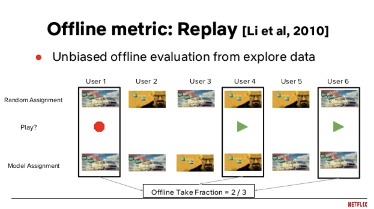
The second problem is that your algorithm will often produce recommendations that are different from the recommendations seen by users in the historic dataset. You can’t supply a reward value for these recommendations because you don’t know what the user’s response would have been to a recommendation they never saw. You can only know how a user responded to what was supplied to them by the production system. The solution to this is a method called replay (Li et al., 2010). Replay evaluation essentially takes your historic event steam and your algorithm’s recommendations at each time step, and throws out all samples except for those where your model’s recommendation is the same as the one the user saw in the historic dataset. This, paired with an unbiased data generating mechanism (such as a randomized recommendation policy), proves to be an unbiased method for offline evaluation of an online learing algorithm.

Netflix’s Jaya Kawale and Fernando Amat provide a nice visual explanation of Replay in these slides from a 2018 conference talk. In this image, there is a production movie recommendation policy (top row) and an offline recommendation policy from a bandit they’re training (bottom). Replay selects the cases where the two recommendation policies agree with each other (the columns with black boxes surrounding them: users 1, 4, and 6), and uses only these play/no-play decisions to score the offline model. So, in this example, the model gets a score of 2/3, since 2 of the 3 matches between the two policies were played.

One drawback to this method is that it significantly shrinks the size of your dataset. If you have \(k\) arms and \(T\) samples, you can expect to have \(\frac{T}{k}\) usable recommendations for evaluating the model (Li et al., 2010). For this reason, you’re going to need a large dataset in order to test your algorithm, since replay evaluation is going to discard most of your data. Nicol et al. (2014) explore ways to improve this via bootstrapping, but for this post I’m using the classic replay method for evaluating the models.

def replay_score(history, df, t, batch_size, recs):
    # reward if rec matches logged data, ignore otherwise
    actions = df[t:t+batch_size]
    actions = actions.loc[actions['movieId'].isin(recs)]
    actions['scoring_round'] = t
    # add row to history if recs match logging policy
    history = history.append(actions)
    action_liked = actions[['movieId', 'liked']]
    return history, action_liked

It’s important to note that replay evaluation is more than just a technique for deciding which events to use for scoring an algorithm’s performance. Replay also decides which events from the original dataset your bandit is allowed to see in future time steps. In order to mirror a real-world online learning scenario, a bandit starts with no data and adds new data points to its memory as it observes how users react to its recommendations. It’s not realistic to let the bandit have access to data points that didn’t come from its recommendation policy. We basically have to pretend those events didn’t happen, otherwise the offline bandit is going to receive most of its data from another algorithm’s policy and is basically just going to end up copying the recommendations reflected in the original dataset. For this reason, we should only add a row to the bandit’s history dataset when the replay technique returns a match between the online and offline policies. In the above function, this can be seen in the history dataframe, to which we only append actions which are matched between the policies.

The final result of this is a complete bandit setting, constructed using historic data. The bandit steps through the dataset, making recommendations based on a policy it’s learning from the data. It begins with zero context on user behavior (an empty history dataframe). It receives user feedback as it recommends movies that match with the recommendations present in the historic dataset. Each time it encounters such a match, it adds this context to its history dataset and can use this as future context for improving its recommendation policy. Over time, history grows larger (although never nearly as large as the original dataset, since replay discards most recommendations), and the bandit becomes more effective in completing its movie recommendation task.

Evaluation Metrics for a Bandit

The last piece you’ll need to evaluate your bandit is one or more evaluation metrics. The literature around bandits focuses primarily on something called regret as its metric of choice. Regret can be loosely defined as the difference between the reward of the arm chosen by an algorithm and the reward it would have received had it acted optimally and chose the best possible arm. You will find pages and pages of proofs showing upper bounds on the regret of any particular bandit algorithm. For our purposes, though, regret a flawed metric. To measure regret, you need to know the reward of the arms that the bandit didn’t choose. In the real world you will never know this! Analyses of this optimal, counterfactual world are academically important, but they don’t take us far in the applied world. We need another metric.

The good news is that, while we can’t measure an algorithm’s cumulative regret, we can measure its cumulative reward, which, in practical terms, is just as good. This is simply the cumulative sum of all the bandit’s replay scores from the cases where a non-null score exists. This is my preferred metric for evaluating a bandit’s offline performance.

It may also be useful to include some metrics that are more meaningful to the specific task that the bandit is performing. If it’s recommending articles or ads on a website, for example, you may want to measure an N-timestep trailing click-through rate to see how CTR improves as the algorithm learns. If you’re recommending videos or articles, you may want to measure measure the completion rate of the views the algorithm generates to make sure it’s not recommending clickbait.

In the case of this dataset, I’ll implement a cumulative reward metric and a 50-timestep trailing CTR, and return both as lists so they can be analyzed as a time series if needed.

cumulative_rewards = np.cumsum(rewards)
trailing_ctr = np.asarray(pd.Series(rewards).rolling(50).mean())

Parting Thoughts

Training a multi-armed bandit using a historic dataset is a bit cumbersome compared to training a traditional machine learning model, but none of the individual methods involved are prohibitively complex. I hope some of the logic laid out in this post is useful for others as they approach similar problems, allowing you to focus on the important parts without getting too bogged down by methodology.

Another thing worth noting is that I’m figuring this out as I go! If you know a better way to go about this or disagree with the approach I’m laying out in this post, send me a note and I’d be interested in discussing this.

Code for this post can be found on github.

Want to learn more about multi-armed bandit algorithms? I recommend reading Bandit Algorithms for Website Optimization by John Myles White.

Get it on Amazon here for $17.77

• 2020 2
• 2019 1
• 2018 2
• 2017 6
• 2016 2