AxeDB: Guitar Pricing Intelligence
New project for studying the used and vintage guitar markets
November 30, 2017
Tanking becomes a hot topic each season once it becomes apparent which of the NBA’s worst teams will be missing the playoffs. Though never explicitly acknowledged, a team with no playoff hopes will sometimes suspiciously begin to decrease the minutes of its starters, leaving its worst lineups on the floor in ways that can only be described as anti-competitive. With playoff glory out of the question, the process of losing by design in pursuit of better draft picks is one of the only remaining ways to extract value from a disappointing season. And so the race to the bottom begins; the losses pile up and fan base turns its eyes to the college talent pool, wondering which member of the upcoming draft class might be the one to turn around the struggling franchise.
The league leadership’s distaste for this strategy of designed awfulness is no secret: it’s boring to watch, bad for advertising revenue, and goes against the ideals of competitive play that Commissioner Adam Silver so adamantly supports. This phenomenon of shedding wins for improved lottery odds is of such high concern to league officials that, beginning with the 2019 draft, lottery odds will be adjusted in order to decrease teams’ incentives to tank. This post is an attempt to understand the value of the draft and of tanking in the NBA, before and after the implementation of the upcoming lottery changes.
Namely, I will address the following questions:
The data for this analysis comes from two different sources. First I manually grabbed all draft results from 1960 to present from basketball-reference.com. The second dataset comes from Kaggle, which provides a dataset of NBA season-level data for each player since 1950. Of this, I kept only the observations since the 1960 season, as anybody who’d played before 1960 wouldn’t be found in the draft pick data. Because the draft has undergone some changes since the 60s, I also removed all picks outside the first and second round, as the draft only has two rounds in its present form.
To determine the value of a draft pick we’ll need to be able to assign it a value. Two of the most commonly used metrics for overall player value are win share (WS) and player efficiency rating (PER).
PER strives to measure per-minute performance while adjusting for pace, taking into account field goals, free throws, 3-pointers, assists, blocks, steals, missed shots, turnovers, and personal fouls. The league average is always equal to 15, values in the 20s indicate star-level performance, and below 10 typically puts a player toward the end of his team’s bench (Wikipedia). Some issues with PER are that it’s measured per-minute, sometimes assigning excessive value to low-minute players and equating them with all stars. It’s also challenging to interpret, since PER points have no direct connection with wins or any other metric. Despite this, PER sees wide use due to its quality of taking multiple facets of the game into account and assigning a single value to a player’s overall per-minute performance. As this metric can become volatile for low-minutes players due to small-sample properties, I ignore PER values for players during seasons in which they averaged less than five minutes per game.
Win Share serves as a convenient response to PER’s flaws. Similar to PER, win shares take into account just about every box score statistic relevant to a player’s performance. WS holds slightly more real-world value, however, in that it’s directly tied to wins. Under Basketball Reference’s system, one team win equals one win share. Players’ contributions are weighed, dividing WS into Offensive and Defensive Win Share (OWS/DWS), where WS = OWS + DWS. Each team’s wins are divided amongst its players according to how much each has contributed on offense and defense. For details on how this is calculated, I suggest reading Basketball Reference’s description here. The all-time single-season record for win shares is Kareem Abdul-Jabbar, who was responsible for 25.4 of the Bucks’ wins in 1971-72. A player on a losing team, on the other hand, has little hope of achieving a high win share, as there are less win shares to distribute throughout the roster.
The last statistic I’ll use in this analysis is an adaptation of sports-reference’s Approximate Value (AV) statistic. Approximate Value takes an existing stat and scales it to weight a player’s best seasons heavier. In my case I’ll front-weight a player’s best win share seasons, adding up 1*(best season) + 0.95*(second best) + 0.9*(third best), all the way down to 0.55*(tenth best). My reason for doing this is that career win shares, as they stand, measure greatness over the span of a player’s career. Some may prefer this, but others will object that this disproportionately rewards players with better longevity and health, which usually can’t be reliably forecast on draft day. Since this is an exercise in the value of draft picks, I find it necessary to include AV as an alternative to WS for this reason. As we’ll see later, AV and WS tell approximately the same story, but I do like that this statistic evens the playing field between a player like Kareem, who had 20 healthy seasons (Career WS 273, AV 144), and Michael Jordan, who only played 15 seasons (Career WS 214, AV 147). It also allows some of the current players to enter the conversation, such as Kevin Durant, currently in his 11th season, who is ranked 35th in career WS (since his career is likely far from over) but 17th in ten-year AV. This adaptation of the AV statistic was inspired by this piece from FiveThirtyEight, which uses AV to evaluate the value of draft picks in the injury-plagued, short-careered National Football League.
As a quick sanity check, let’s see who some of the all-time greats are according to these three measures.
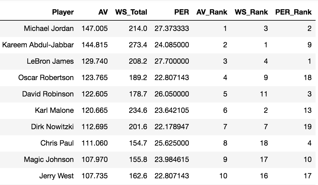 Table 1: Top Ten Players Drafted Since 1960 According to Approximate Value (AV)
This looks about right. Career Win Share rewards greatness over the course of a career, Approximate Value rewards greatness at a player’s peak over a ten year period, and PER rewards a player’s average efficiency. Accordingly, all players on this list are deserving of legend status, AV rewards the short-careered all-time greats such as David Robinson and Magic Johnson, and PER rewards those who packed the most productivity into their time on the floor.
Since PER doesn’t appear to match the other two measures too closely, we can double-check that these metrics tell roughly the same stort using a measure called Kendall Correlation. Kendall correlation is a measure of the pairwise similarity or dissimilarity of two sets of rankings. A value close to 1 indicates near-perfect agreement between the ranking systems, close to -1 indicates near-perfect disagreement, and close to 0 indicates little-to-no relationship between them.
Here we see a correlation of 0.89 between AV and WS, of 0.61 between AV and PER, and of 0.58 between PER and WS. So while AV and WS are much more similar to one another than either of these two metrics are to PER, they’re all similar enough accept as valid ranking metrics, significantly positively correlated with P<0.001 while clearly succeeding in the task of identifying high achievers.
With this in mind, we should now feel comfortable accepting that these are useful metrics that tell similar but non-identical stories of player value. Taken holistically, these should be all we need to evaluate the values of positions in the draft.
Given each player’s draft position, AV, WS and PER, the first step is to see how many points of each of these metrics can be expected from each draft position.
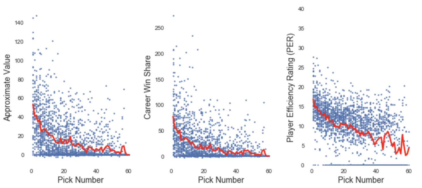 AV, WS, and PER by Pick Number, with Means Shown in Red
The above plot shows two of the things we’d expect: a downward trend in player value as the draft progresses, and a relatively high variance in player value at each pick. The relationship between pick number and each of these player-ability metrics is highly significant, with each having an absolute pearson correlation of >0.41 with P<0.001. What’s more interesting, however, is that each of these three relationships appears to be nonlinear in a similar way, indicating a potentially complex relationship between tanking and draft value. Also worth noting is that many players selected within the last 10 picks of their respective draft classes had negative PER ratings, which aren’t shown on the above figure but can be inferred by the average (red) falling below the visible points on the scatter plot.
We’ll need to take a step beyond these simple averages in order to give this relationship a more believable functional form. It defies logic to say that the 8th pick, for example, is worth 3 more win shares than the 7th pick. For this reason I fit a fifth-order polynomial to this data to enforce the qualities of smoothness and having pick values consistently decrease according to their position in the draft.
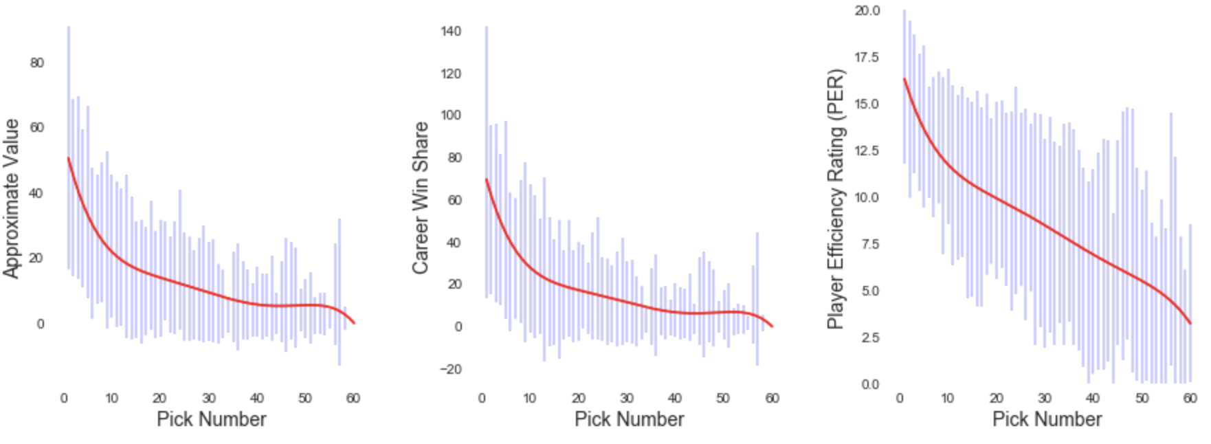 Smoothed Expected Values for Each Pick Number. Error Bar Represents One Standard Deviation in Either Direction.
The outputs of these smoothed functions are what I’ll use for the rest of this analysis when referring to pick values. The relationships between WS, AV and pick number resemble exponential decay until these values fall off in the draft’s final picks. Expected PER decreases in a a much more linear fashion once outside the top ten picks, falling off similar to AV and WS at the tail end of the draft.
The error bars in these plots represent standard deviations from the mean, meaning that 68.27% of values lie within these ranges. For WS and AV the standard deviations decrease in the draft’s later picks, indicating that as players get worse we can become more confident what their output will be. PER, on the other hand, gets less stable in the tail end of the graph. This is because PER is measured per minute, meaning that low-minutes players will sometimes have illogical ratings due to small sample properties. All three measures see higher standard deviations in the draft’s final two picks due to the fact that the league hasn’t always had 30 teams.
The expected AV, WS, and PER for each draft position is shown below.
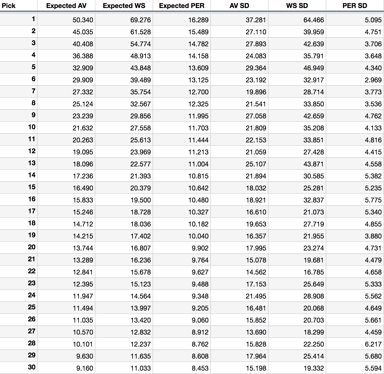
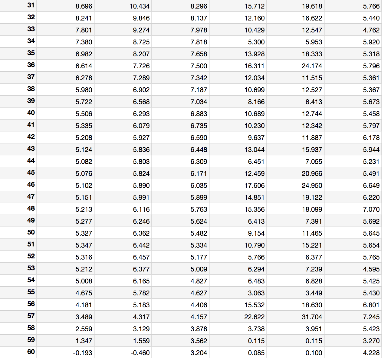 Table 2: Expected Values and Standard Deviations of Each Pick Position
Before getting into tanking, the above numbers are valuable to teams and worth a closer look. With these values alone we can objectively evaluate the quality of a draft-day trade that involves only draft picks.
Table 3 does exactly that. The first example reads as follows:
In 2017 the Kings received picks 15 and 20 from the Blazers in exchange for the 10th pick. The picks received by the Kings were worth an expected 37.19 career win shares and combined 20.54 PER, while the Blazers’ pick was worth an expected 29.86 win shares and 11.70 PER. The Kings came out on top in this trade, netting an additional 7.33 expected win shares and 8.84 points of PER.
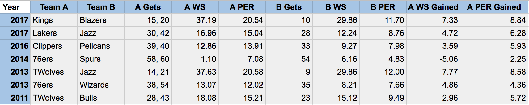 Table 3: WS and PER Gained/Lost in Recent Draft Day Trades Involving Only Draft Picks
The lesson learned here? Much like Richard Thaler teaches us about NFL draft pick valuations, NBA teams should trade down in the draft far more often than they currently do. The 76ers and Timberwolves appear to be on to this strategy, but the rest of the league is yet to follow suit.
This same analysis can be extended to trades involving players and future draft picks, but it involves a little more work and uncertainty. Some thoughts on how to take into account the three non-draft pick assets that get tossed around on draft day:
Under its current rules, the lottery provides the league’s worst 14 teams a chance at winning each of the first three picks. After the first three picks are determined according to randomly generated numbers, each of the following picks is assigned to the worst remaining team. Outside the worst 14 teams, draft position is predetermined according to the inverse of a team’s rank within the league. Each team’s odds of receiving each lottery placement are shown below in highlighted cells, where rows represent inverse rankings (i.e. rankings in terms of how bad a team was) and columns represent pick numbers.
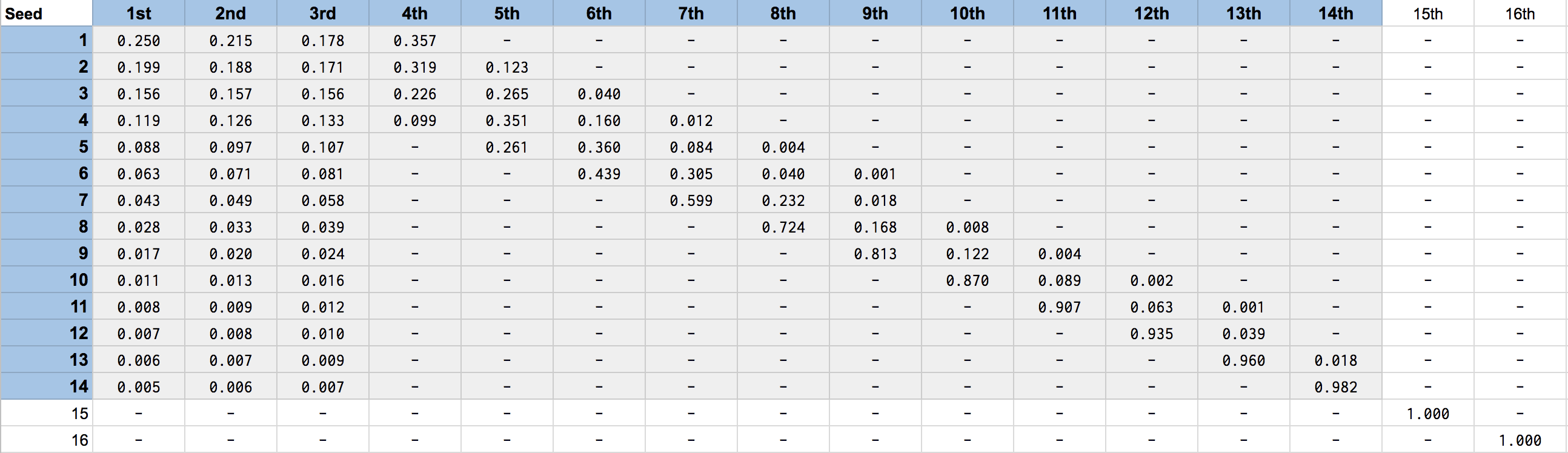 Table 4: Odds of Winning Each Pick by Inverse Record Ranking. Lottery Picks are Highlighted.
Outside the lottery (picks 1 - 14), the 15th worst team has a 100% chance of earning the 15th pick, the 16th worst team gets the 16th pick, and so on down the line. Second round picks are unaffected by the lottery, meaning that the worst team gets the first pick of the draft’s second round regardless of whether they won the lottery for the first pick overall. For more detail on this process, Wikipedia has a nice overview
Taking the above lottery odds and earlier-discussed valuations of each pick position, it’s easy to combine these in order to place a value on each end-of-season rank in terms of its expected draft-day value.
Starting with Table 4’s lottery odds, multiply the percentages in each column by the value of the corresponding pick number from Table 2. Once pick value and probability have been multiplied together for all 30 teams and 60 picks (most of these values will be zero, since there’s no uncertainty in the assignment of picks 15 - 60), take the sum of these values for each end-of-season ranking to obtain its expected draft-day value in terms of draft picks. Stated a different way, this is simply the dot product of the (ranking x pick probability) matrix and the vector of pick valuations.
Two examples to illustrate this:
Worst team in the league: 0.250(69.28) + 0.215(61.53) + 0.178(54.77) + 0.375(48.91) + 1.000(10.43) = 68.19 expected career win shares
Tenth worst team: 0.011(69.28) + 0.013(61.53) + 0.016(54.77) + 0.870(27.56) + 0.089(25.61) + 0.002(23.97) + 1.000(6.29) = 35.03 expected career win shares
Below are the expected values of all 30 end-of-season rankings in terms of win shares, approximate value, and points of player efficiency rating. As we’d expect, these show similar patterns to the relationships between pick number and value. The two main differences are that these curves are shifted vertically and compressed, since the values now include both first and second round picks, and that they’re flatter, since each of the bottom 14 ranked teams has a chance at the top three picks. The exact values from these plots are shown in the next section in Table 5.
![]() Expected AV, WS, and PER of Each End-of-Season Ranking
Expected AV, WS, and PER of Each End-of-Season Ranking
With the value of each end-of-season ranking established, we’re finally able to face the question this analysis set out to answer: what’s to gain from tanking? Should a team act anticompetitive in order to improve its lottery odds?
The value of tanking one position in the league standings is the difference between the value of a team’s current ranking and the value of falling one place closer to the bottom of the league. These values come from the weighing of draft pick odds and their values discussed in the previous section. These season-end rankings’ values are shown alongside their “tanking values” in Table 5, where a tanking value is defined as the difference between one end-of-season ranking’s expected draft day value and that of the next worse ranking. These values are positive for all rankings and for all three measures of value, with no tanking value being assigned to the worst team in the league since there’s nowhere to fall for a team that’s already hit rock bottom.
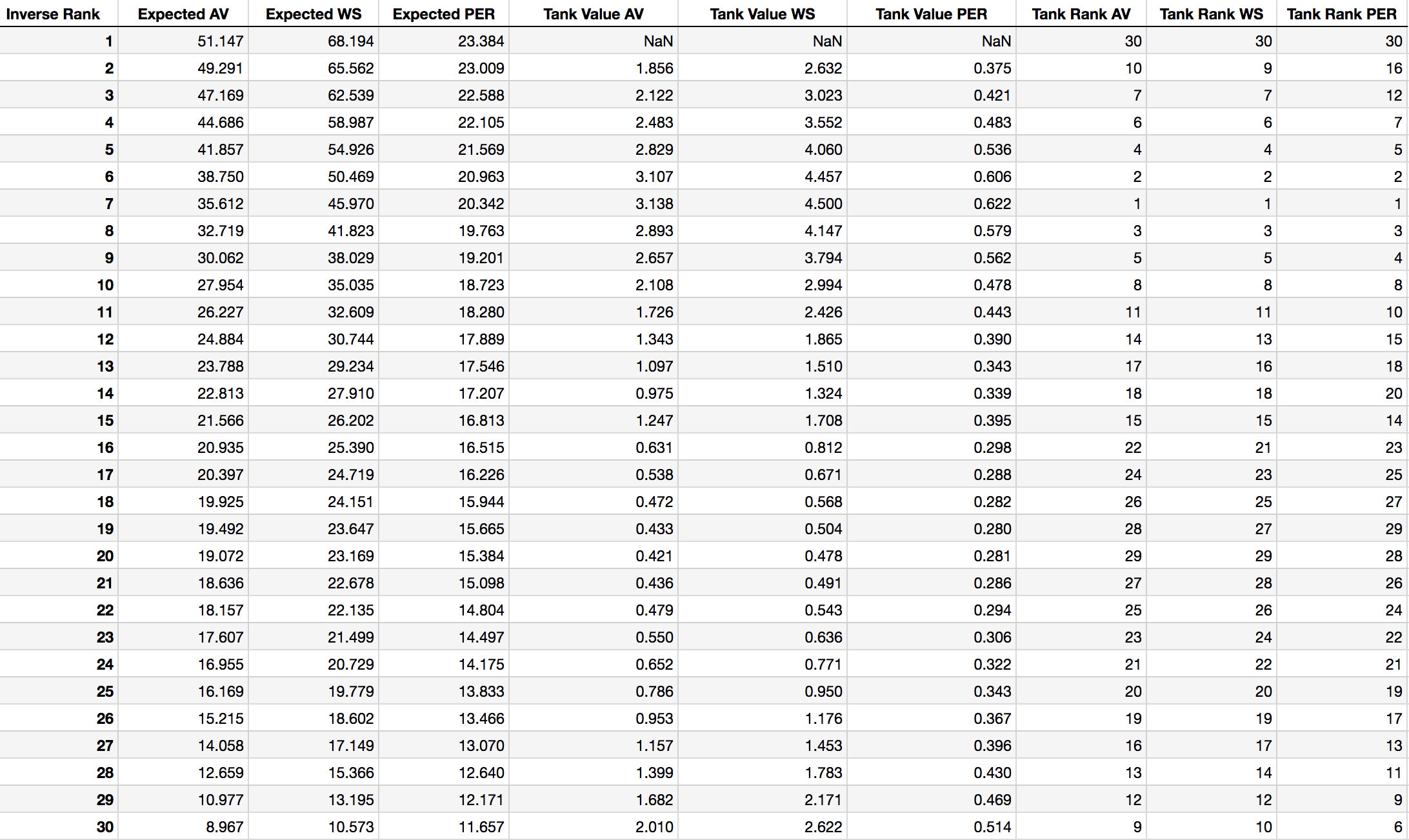 Table 5: Expected Value and Tanking Opportunity of Each Inverse Team Ranking
Ranking these positions by how much a team would gain by tanking one additional spot shows an interesting relationship. For all three measures of value, the worst non-lottery teams have the least to gain by tanking. It’s also interesting to see that teams expected to be placed in the middle of the lottery have more to gain than those closest to the league’s worst ranking. If we discard playoff-eligible teams from these rankings, the sweet spot for tanking is ranks five through eight. It’s valuable to tank for teams of all ranks, of course, but these mid-lottery rankings are where we see that teams have the most to gain from losing a few additional games.
To understand this relationship better, let’s plot tanking value against inverse league rank. Again, by “inverse rank” I’m referring to the opposite of a team’s place in the league standings, where the league’s worst team has an inverse rank of one, the second worst team has an inverse rank of two, and so on.
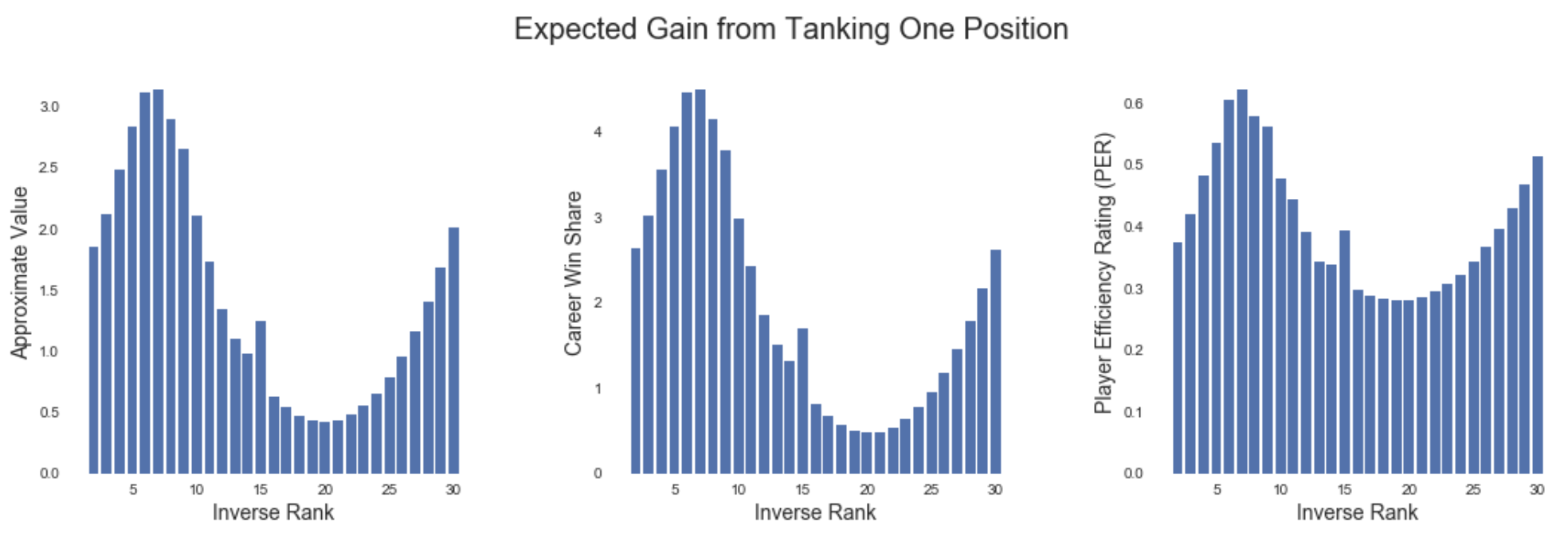 Draft-Pick Value of Falling One Position in the Rankings
After seeing this visually, a few additional things become apparent about tanking. First, there’s a significant increase in tanking-value for the league’s 15th-worst team. This is because Falling from 15th to 14th worst enters a team into the lottery, giving them a chance at the much-more-valuable first, second, third pick, as well as a guarantee of the slightly-more-valuable 14th pick if the better options don’t pan out. Second, the power-law nature of the value of draft picks also shows through in this. Tanking becomes increasingly valuable as rank improves for the league’s best teams, since a disproportionate amount of the draft’s value tends to come from the first half of the first round.
Since no sensible team in the playoff hunt is going to throw wins for a better draft position, we can safely ignore the right-hand side of these plots. What’s most important is that the relationship between ranking and expected draft-pick value is nonlinear in a way that gives the league’s fifth through eighth worst teams the most to gain from losing games down the stretch.
Turning to the real-world value of falling in the rankings, however, these values individually aren’t shocking. Falling one position in the league rankings is worth an additional 0.62 points of PER, 4.35 career wins, and 3.11 approximate value points at best. This is hardly going to turn around a franchise.
A formal long-term strategy of tanking, on the other hand, might be a different story. Imagine a team whose non-tanking league ranking is seventh worst. If this team were to adopt a policy of end-of-year tanking for just two seasons in a row, falling three spots each year, they would gain an impressive 3.53 points of PER, 26.21 career win shares, and 18.28 points of AV. Stretch this out to a third year of designed awfulness and you have 5.29 PER, 39.32 WS, and 27.42 AV, all in addition to the already-high expected values of their mid-lottery odds before tanking. Suddenly this looks valuable, and it’s not far off from what the 76ers have been accused of doing in recent seasons.
The NBA is aware of this strategy, and in September 2017 came to an agreement with the Board of Governors to change the lottery’s odds in a way that disincentivizes the practice of tanking. The first major change is that, starting 2019, the league’s three worst teams will have identical odds of winning the first pick rather than the current odds which favor worse records. The second change is that lottery teams will be able to fall further down in the draft than is possible under the current rules. Where the worst possible outcome for the league’s worst team is currently the fourth overall pick, starting 2019 they will be able to fall to as far as fifth.
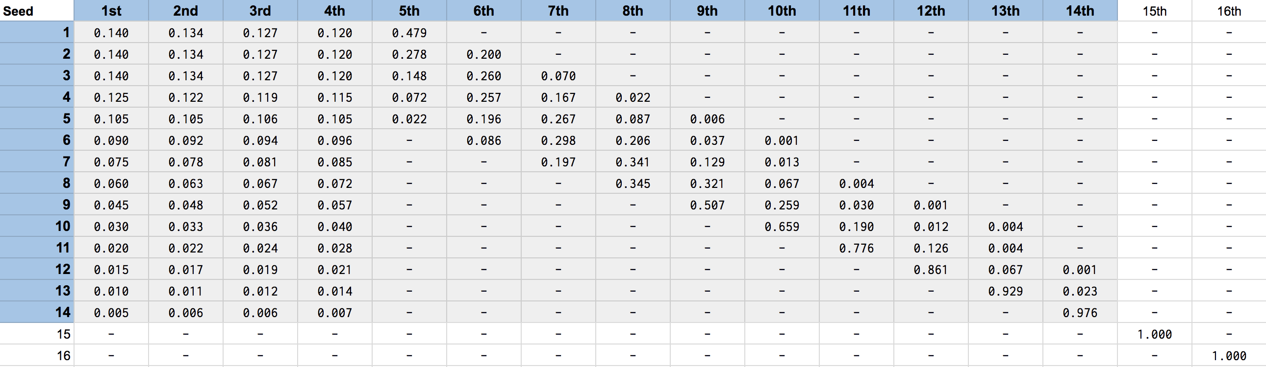 Table 6: Lottery Odds Effective 2019
So the rewards for being among the league’s absolute-worst will decrease, and the worst-case scenario for these same teams also becomes slightly less desirable. Will this be enough to stop teams from tanking? Let’s see how severely these changes affect each end-of-season ranking and tanking value.
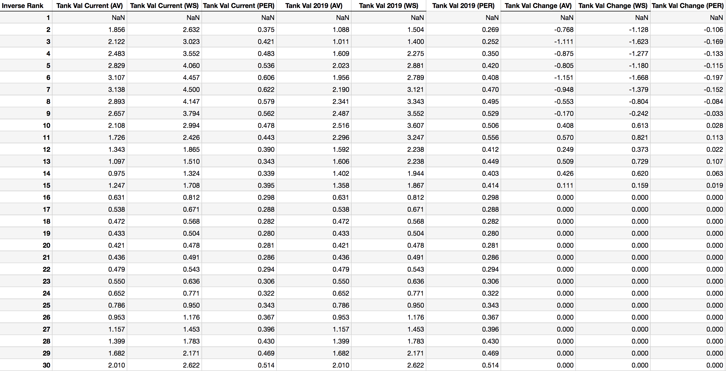 Table 7: Tanking Values under Current and Future Lottery Odds
Table 7 shows that the values of each end-of-season ranking will remain similar in magnitude after the new lottery rules go into effect. The values of tanking for the worst nine teams, however, will decrease, while these values increase for the five best lottery teams (ranks 10 - 14). Non-lottery teams’ odds are unaffected, as there’s no uncertainty surrounding their draft positions.
![]() Value of Tanking Before and After Lottery Change
Value of Tanking Before and After Lottery Change
Plotting these new values against the current ones, it’s clear that the relationship between season-end ranking and draft value is visibly flatter under the new lottery. For those taking the anti-tanking stance, this is a good thing. For those who believe that the league’s worst teams deserve better lottery odds in order to ascend from mediocrity, this is a bad thing.
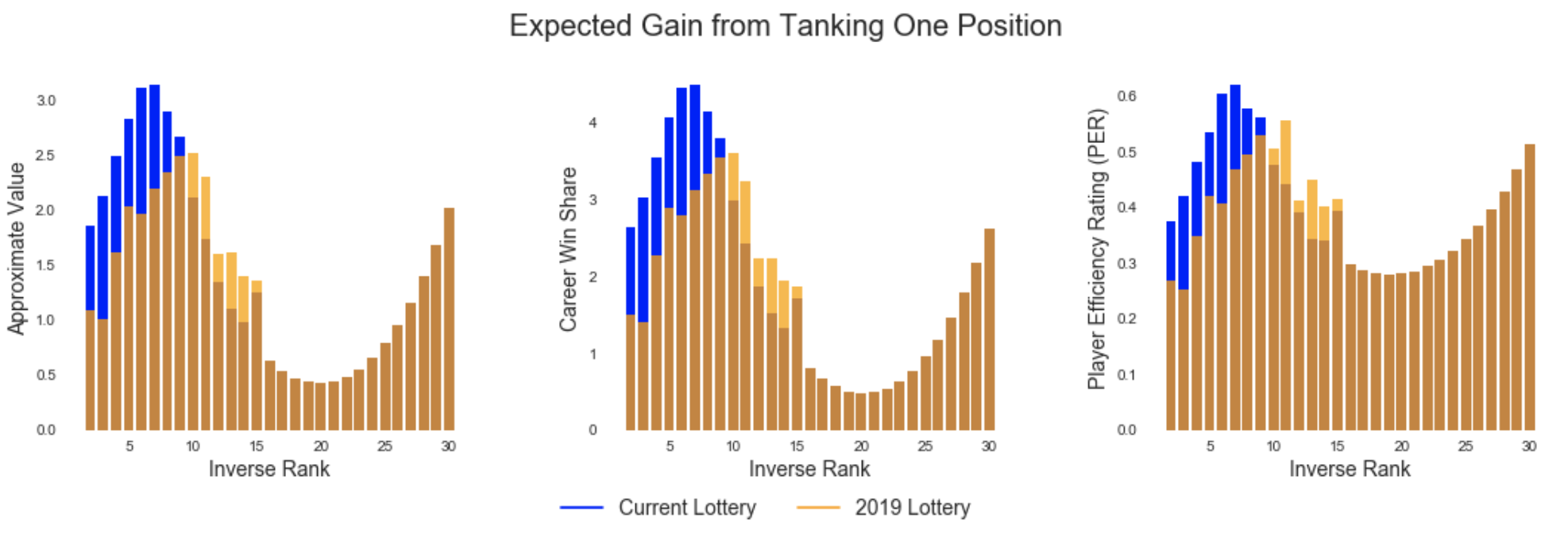 Tanking Values Before and After Rule Change
Plotting tanking values before and after this change shows a similar story. The new odds make it less valuable for inverse ranks 1 - 9 to lose games, more valuable for ranks 10 - 14, and leave ranks 15 - 30 untouched.
A final question worth answering is how this all nets out. At the league level, will it be less valuable to tank than under the current rules? The answer to this is a simple “yes.” The sum of the differences in tanking value for each rank between the old and new lottery system is negative in terms of AV, WS, and PER. Specifically, the new lottery odds result in 0.64, 5.98, and 4.10 point drops in available PER, WS, and AV to be gained from tanking respectively. Tanking will still be valuable to the league’s worst teams, but the incentive to do so has been ever-so-slightly reduced, and will be shifted slightly toward teams that are still in the playoff hunt (the 10th - 14th worst teams). As a result, one can expect a slightly more competitive league going forward.
New project for studying the used and vintage guitar markets
This post explores four algorithms for solving the multi-armed bandit problem (Epsilon Greedy, EXP3, Bayesian UCB, and UCB1), with implementations in Python ...
Multi-armed bandit algorithms are seeing renewed excitement, but evaluating their performance using a historic dataset is challenging. Here’s how I go about ...
An analysis of auction dynamics in client-side header bidding
Using machine learning to predict strategic infield positioning using statcast data and contextual feature engineering.
A quick tutorial on fetching MLB win-loss data with pybaseball and cleaning and visuzlizing it with the tidyverse (dplyr and ggplot).
Tanking becomes a hot topic each season once it becomes apparent which of the NBA’s worst teams will be missing the playoffs. In this post I address the valu...
I’ve been borderline obsessed with the eephus pitch for some time now. Every time I see a player pull this pitch out of their arsenal I become equal parts ex...
For the past three months I have had the exciting opportunity to intern as a data scientist at Major League Baseball Advanced Media, the technology arm of ML...
Throughout my baseball-facing work at MLB Advanced Media, I came to realize that there was no reliable Python tool available for sabermetric research and adv...
A collection of some of my favorite books. Business, popular economics, stats and machine learning, and some literature.
Each cup of coffee I have consumed in the past 5 months has been logged on a spreadsheet. Here’s what I’ve learned by data sciencing my coffee consumption.
Literature is a tricky area for data science. Think of your five favorite books. What do they have in common? Some may share an author or genre, but besides ...
Probabilistic modeling on NFL field goal data. Applying logistic regression, random forests, and neural networks in R to measure contributing factors of fiel...